The Instagram Challenge: how to unshred an image using Python

November 15th, 2011

In retrospect, this code isn't very good, but writing down my thought process and putting it into the world landed me a job at Instagram as a 20 year old kid. I'm thankful the team saw potential and took a bet on me. If you dedicate yourself to a craft, you'll cringe at your work from just a few years ago: that's growth!

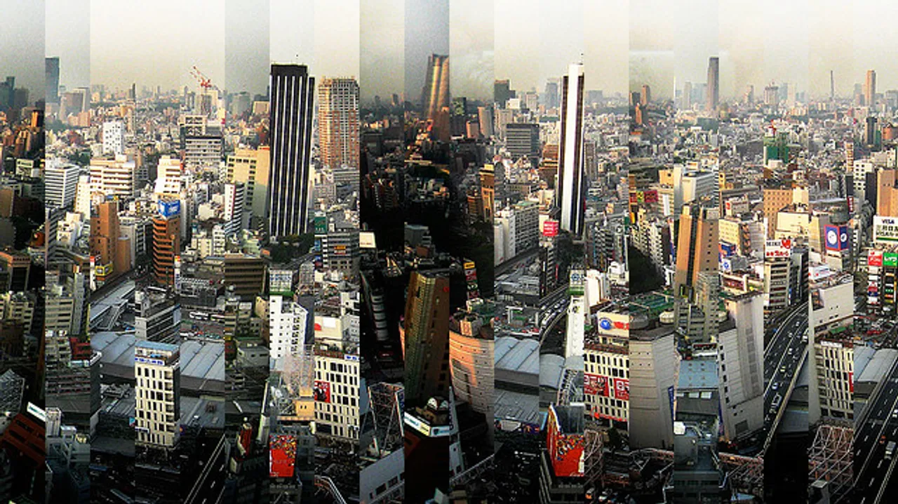
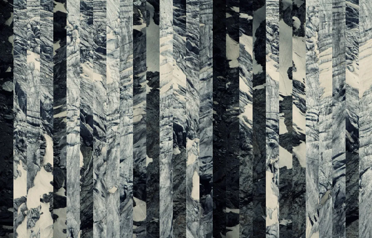
Instagram recently doled out a photo challenge: to un-shred a shredded image. I decided to give it a shot. Let’s see what we can do in under 100 lines of Python…

A Naive Attempt

Let’s start with the simplest un-shredding problem. We’ll begin with an evenly sliced image with a known number of pieces (n). These pieces have 2n edges. A successful un-shredding requires making n-1 matches between edges. If we can make these matches, we can reconstruct the image.

Naive Matching: The most basic matching attack is greedy. We can pick a single piece with which to start, then find a matching right-hand neighbor, find the neighbor’s matching neighbor, and so on until we’ve made n-1 matches.

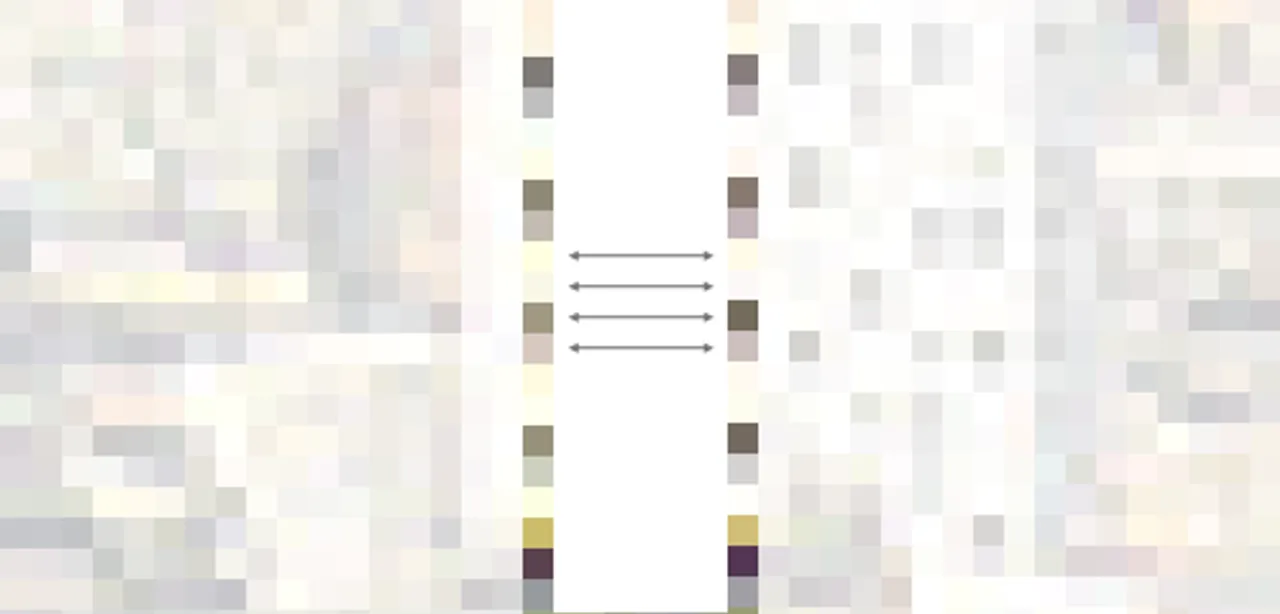
Naive Comparison: The simplest approach for comparing two pieces will be to compare two pixels at a time. Since we’re looking to fuse two pieces together, we can iterate down the pieces edges’ and compare pixels as we go:

To compare two pixels, we’ll calculate the distance in color between them. RGB color space is 3D space, so it looks like this:

Note: We can do this for any color space, including ones with alpha channels.

Iterating down the sides of the two pieces (height h), we can generate an aggregate delta score for the two edges. Minimizing the delta means finding a match of “best fit”.

class Piece:
	def __init__(self, img):
		self.image = img
		self.edges = img.crop((0, 0, 1, HEIGHT)).getdata(),
			img.crop((img.size[0] - 1, 0, img.size[0], HEIGHT)).getdata())

def compare_pixels(p1, p2):
	distance = 0
	for c in range(3):
		distance += pow((p1[c] - p2[c]), 2)
	return math.sqrt(distance)

def edge_delta(e1, e2):
	edge_delta = 0
	for p in range(len(e1)):
		edge_delta += compare_pixels(e1[p], e2[p])
	return edge_delta / LIMIT / HEIGHT

Here’s our new image, generated with 42 lines of Python:

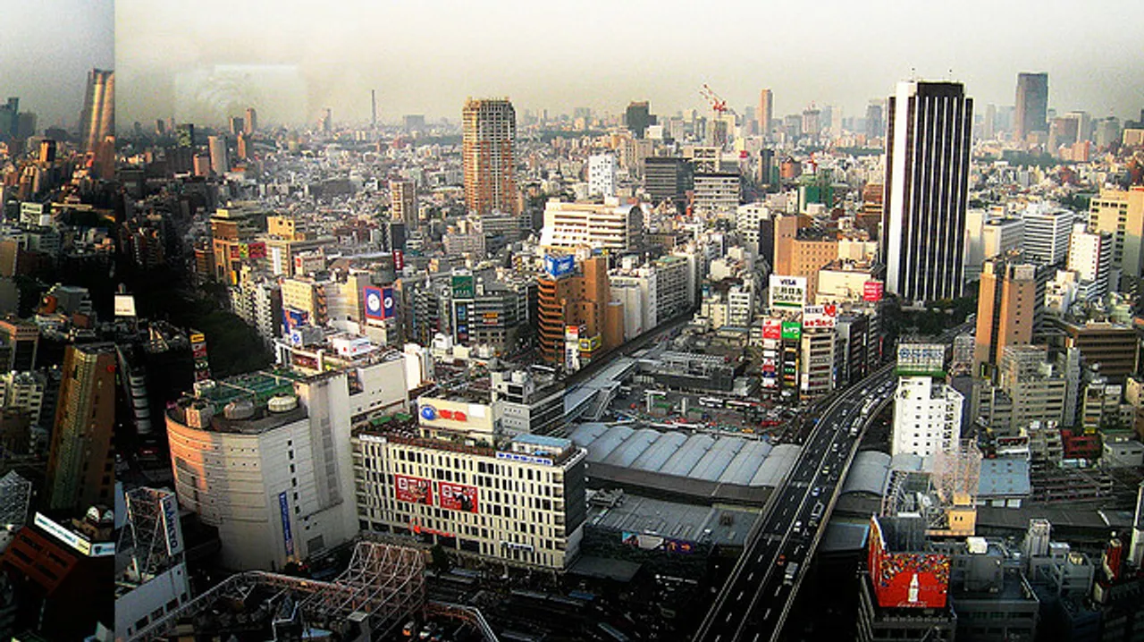
Close. There is one glaring problem here: our greedy matching algorithm only works if we start with the left-most piece. Otherwise, we’ll ultimately force a match that doesn’t exist.

Smarter Matching

Every piece has at least one neighbor. However, not all pieces have two (i.e. edge pieces). One piece lacks a left neighbor and another is missing a right neighbor. So a truly greedy algorithm is not the best approach.

A better method would be to choose a piece at random and propose both a left match and a right match, but only pick the best one. We can determine which match is strongest (minimum delta), then fuse the stronger match while leaving the other alone. If we proceed this way, we will never force an unnecessary match. Instead, our two least-similar edges will remain unmatched.

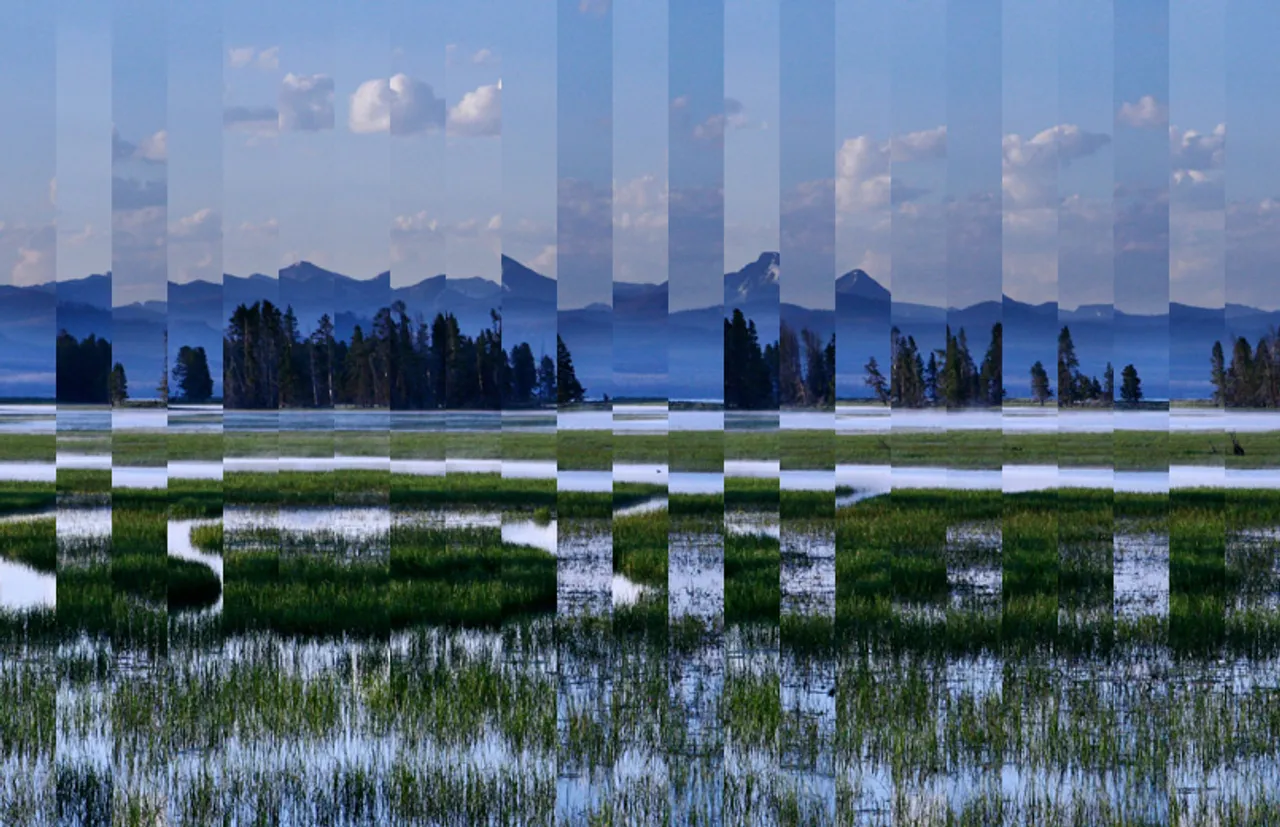
What happens when we implement this new matching scheme? (+12 lines)

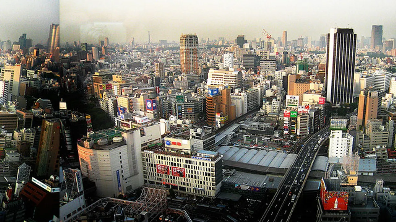
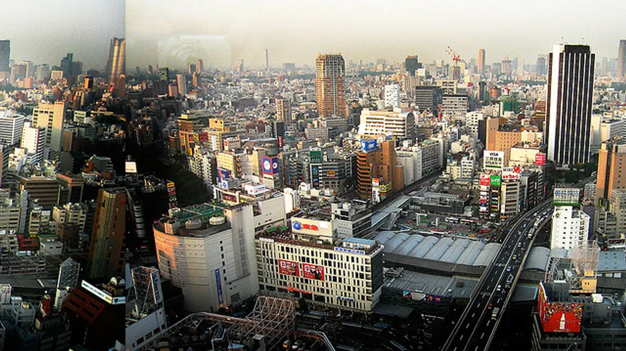
What the heck! After four iterations, our program decides to pick the center seam as the better match. Looks like our comparison algorithm needs work.

Smarter Comparison

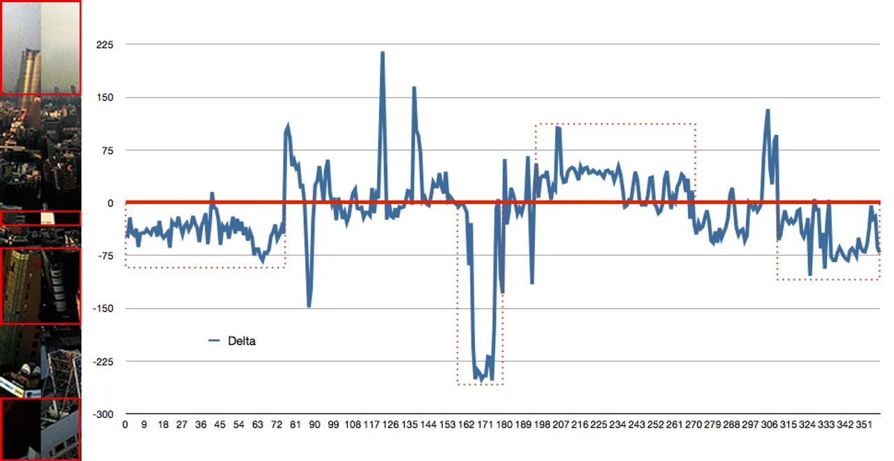
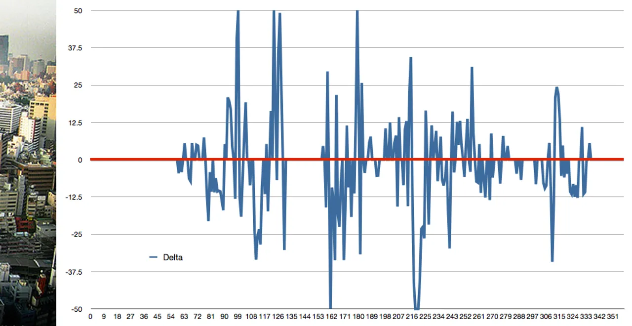
Let’s not guess about the weaknesses of our algorithm. Instead, let’s look at the data. Here is a graph of the color difference between the two edges making our gruesome seam. The x-axis depicts pixels, top to bottom:

False Positive #1:

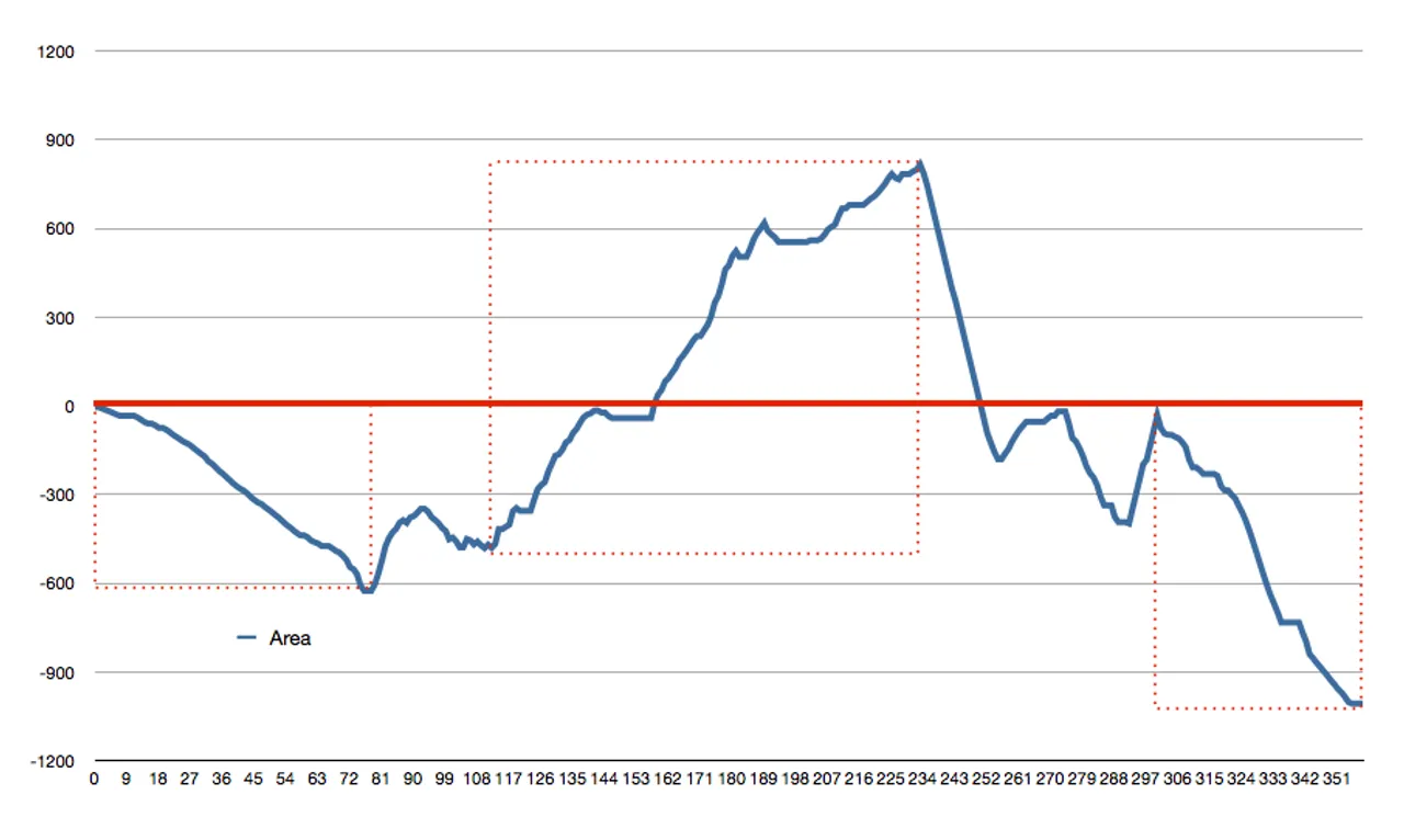
And here’s a graph depicting the delta score of a valid match that our algorithm deemed poor:

False Negative #1:

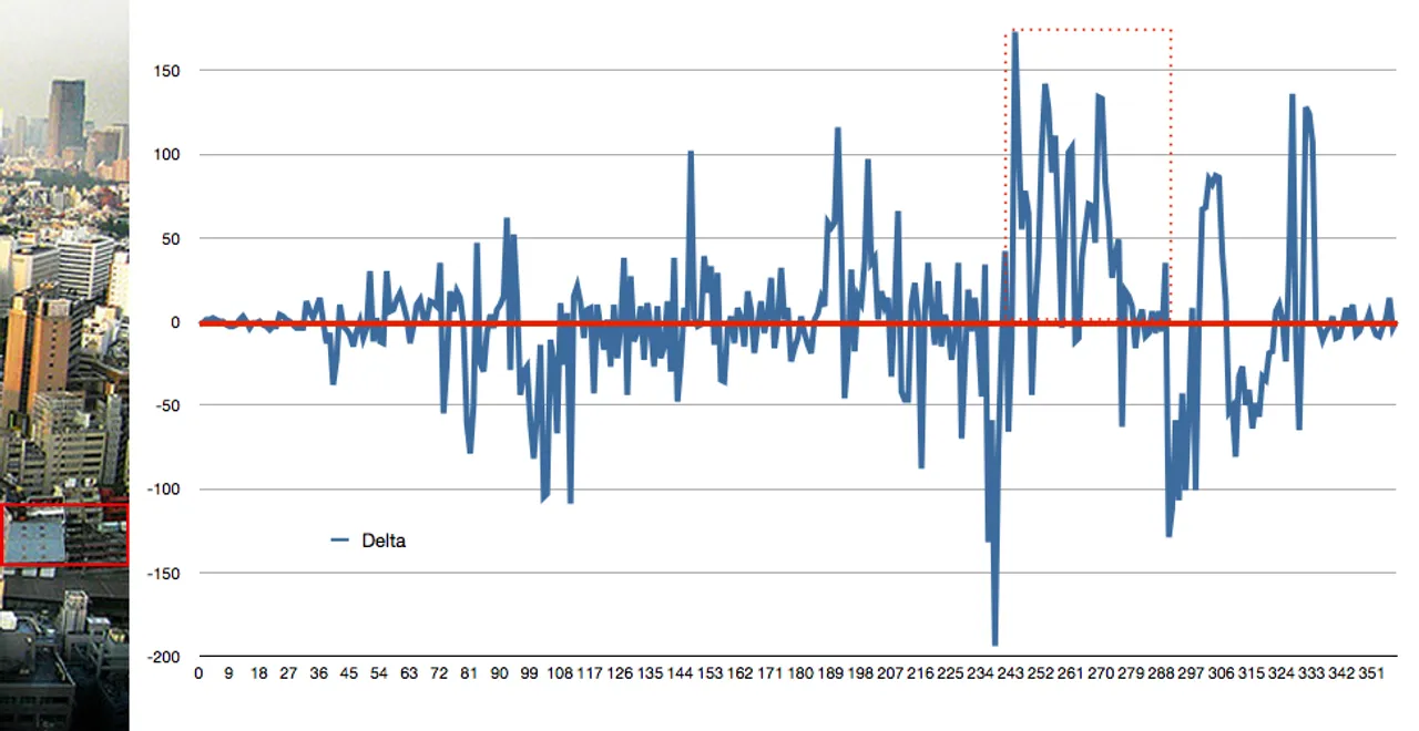
The first graph shows consistent differences. For instance, the sky in the left piece trends darker for about 20% of the image. Similar trends can be seen in the lower portion of the image. Conversely, the second graph shows few trends. Instead, differences are erratic, but image noise and the busyness of the scene make for large discrepancies at an individual pixel level.

We can make some very simple changes to our algorithm to make it better. In general, we should consider the RGB distance between colors to be a faulty measure. Instead, we should work to calculate the perceived difference between colors as seen by humans.

CIELab: The CIELab color space was created to match the “perceptual nature” of color. Changing our color space from RGB to CIELab will help to compute more perceptual “distances” between pixels.

Similar is same: Certain color differences are negligible to the human eye and some random differences must be expected in images (due to noise and artifacts). We’ll implement a threshold to ignore these small variances when computing our delta.

Black and white is blue and white: Once color differences reach a certain limit, we can consider the variance to be “fully significant.” Implementing an upper limit will lessen the dramatic effect that a few severe variances in color may have on our delta.

class Piece:
	def __init__(self, img):
		self.image = img
		self.edges = (rgb_to_cie(img.crop((0, 0, 1, HEIGHT)).getdata()),
			rgb_to_cie(img.crop((img.size[0] - 1, 0, img.size[0], HEIGHT)).getdata()))

def clip(delta):
	if abs(delta) < THRESHOLD: delta = 0
	elif abs(delta) > LIMIT: delta = math.copysign(LIMIT, delta)
	return delta

def compare_pixels(p1, p2):
	distance = 0
	for c in range(3):
		distance += pow((p1[c] - p2[c]), 2)
	return clip(math.sqrt(distance))

How do these basic changes fare? (+13 lines.)

A little different, but we still haven’t solved our problem. Let’s look at the new graphs (CIELab color variances with upper and lower bounds):

False Positive #2:

False Negative #2:

Again, the first graph shows some trends while the second suggests normal chaos. Pixel-level comparisons just aren’t going to be enough. We need to construct a metric for measuring trends.

Finding Patterns

The graphs above are hard to read, so let’s make them a little clearer. Instead of graphing the pixel-by-pixel deltas, let’s graph the aggregate sum of the variances. E.g. let’s graph a rough integration of our pixel variances:

False Positive #2 (Integrated):

False Negative #2 (Integrated):

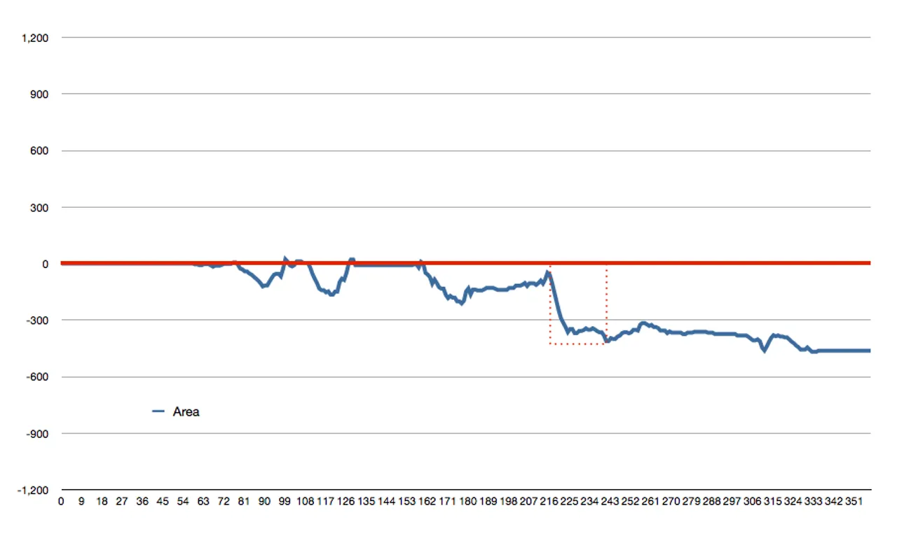
Hey hey! We’re on to something!

We can see a very clear pattern in the false positive now. It looks like we could take the absolute area under this integration curve for our metric. But that’s only sorta-smart. While such a metric would separate large trends from small ones, it still wouldn’t minimize the effect many small discrepancies might generate. So let’s be smarter…

When random chaos generates apparent trends, these “trends” don’t last long. We can create a better metric for finding real trends by considering historic values. My proposition:

def edge_trend(e1, e2):
	edge_trend = 0
	for c in range(3):
		bucket = []; bucket_count = 0
		for p in range(len(e1)):
			diff = clip(e1[p][c] - e2[p][c]) / 3.0
			bucket.append(diff)
			bucket_count += diff
			if len(bucket) > BUCKET_SIZE:
				bucket_count -= bucket.pop(0)
			edge_trend += abs(bucket_count) / BUCKET_SIZE
	return edge_trend / LIMIT / HEIGHT

When comparing edge pixels, we should store a bucket of recent variance information (say the latest 10%). We can measure the significance of ongoing trends by tallying up the historic data as we move down the edge. This will minimize severe, erratic ups and downs (they’ll flatten out over recent history) while capturing large holes and mounds.

Putting it Together

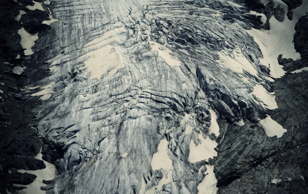
What happens when we combine a basic comparison routine, a more “perceptive” color space, upper and lower bounds, and a historic trend metric?

Well, 88 lines of Python give us this:

Extra Credit

We’re not done! Let’s get some bonus points…

Rotation: We shouldn’t need to arrange our shredded pieces before stitching them back together. We can quickly add additional comparisons for rotated pieces.

class Match:
	def __init__(self, edge, side, piece):
		self.edge = edge
		self.piece = piece
		normal = compare_edges(edge, piece.edges[not side])
		flipped = compare_edges(edge, piece.edges[side][::-1])
		self.flipped = (flipped < normal)
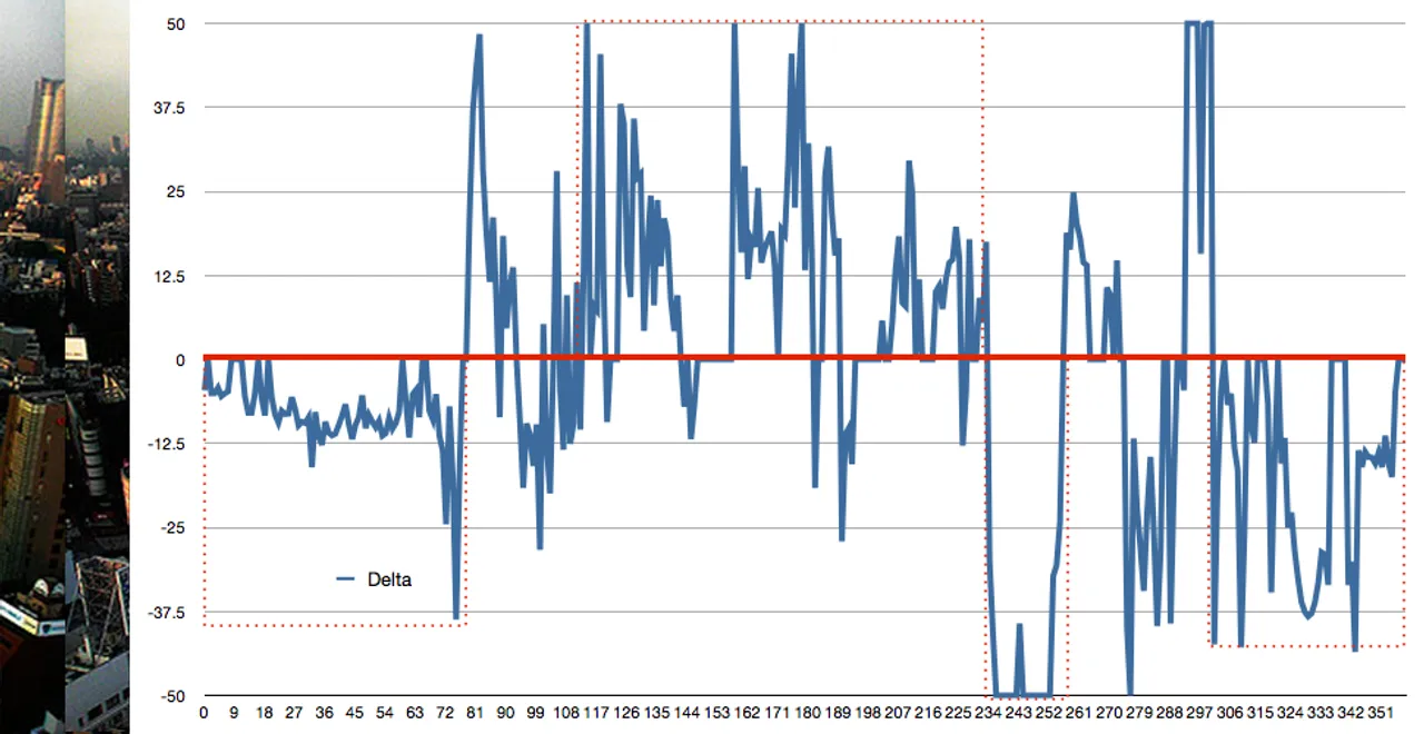
		self.score = min(flipped, normal)

Detecting Shreds: So far, we’ve been hard-coding the number of strips that comprise our image. But it isn’t hard to determine this for ourselves. Take a look at our edge comparison metric as we scan the image horizontally:

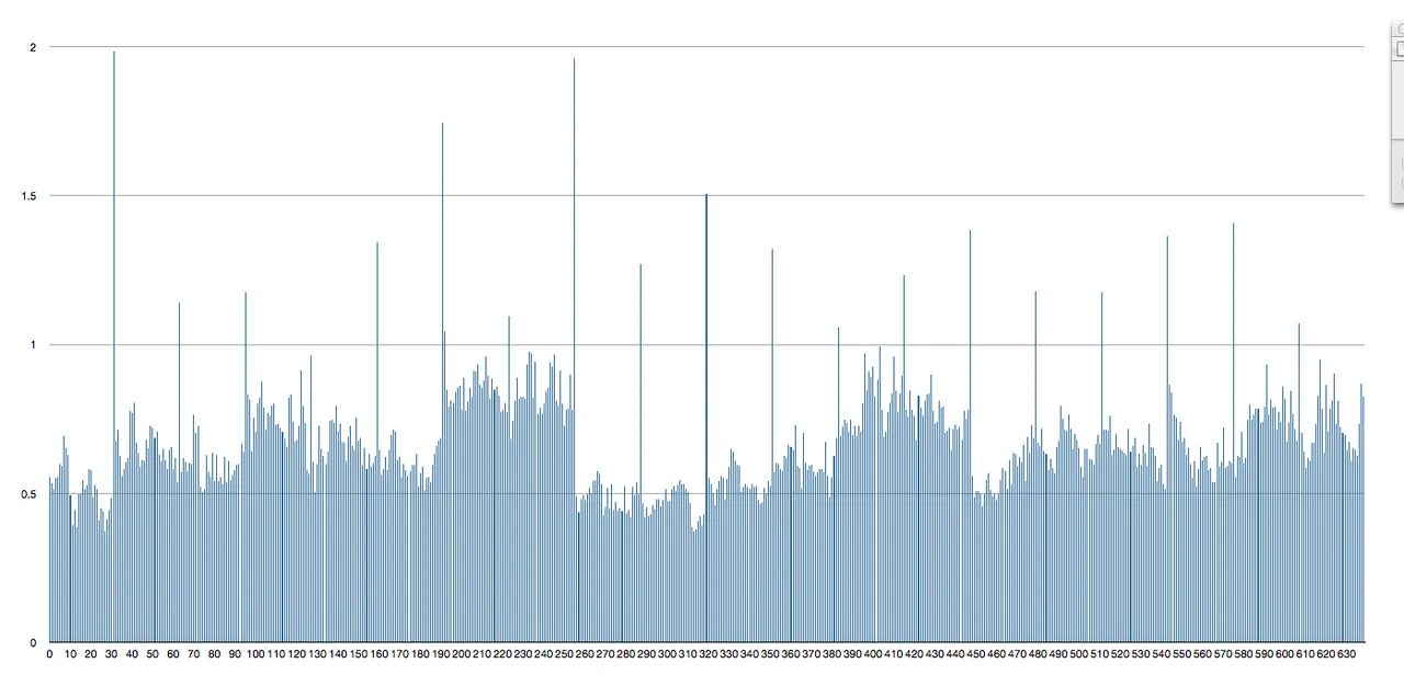
Let’s find a good value for a “significant deviance” (say 1.0) and pull out the relative locations of scores above this threshold:

breaks = []; last_c = 0
for c in range(WIDTH-1):
	delta = compare_edges(column(c), column(c + 1))
	piece_size = c - last_c
	if delta > CUT_VALUE and piece_size > MIN_BREAK:
		breaks.append(piece_size); last_c = c
breaks.sort()
PIECE_WIDTH = breaks[len(breaks) / 2]

[31,32,32,32,32,32,32,32,32,32,32,32,32,32,32,32,32,32,32]

Obviously, this list isn’t completely perfect. But considering the fact sky scrapers have edges, it’s pretty good. Since the shreds are uniform, we can just use the median to accurately determine our shred width.

Conclusion

We’ve written a mere 99 lines of intelligent code capable of un-shredding almost any input image.

Possible Extensions

For large images, we may want to consider an edge to be wider than a single column of pixels. We could apply some basic reductions to our edge data to minimize noise and use a less volatile sample.

It would be also cool to use outline detection to stitch a shredded image back together. Theoretically, we could measure the y-intercept and gradient of contrast lines approaching an edge. We could then give our matches “bonus points” if they fuse an outline together.

Mentioned in:

My writing

Ryan’s notes